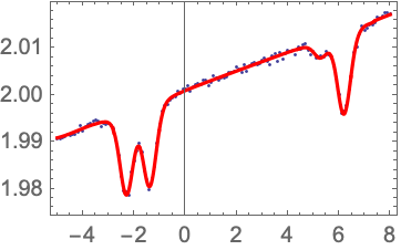
Linear Absorption Fitting
The density of an atomic vapor can be determined by measuring the absorption of weak resonant light. In this example we use the LinearAbsorption function from the AtomicDensityMatrix package along with values from the AtomicData database to construct a fitting function for linear absorption on an alkali D-line. Fitting a linear absorption spectrum with this function allows the atomic density to be extracted.
We define the Doppler width as the magnitude of the Doppler shift corresponding to the most probable speed in the Maxwell velocity distribution.
LinearAbsorption[sys,ω,ΓD,ΓP] finds the absorption by system sys with Doppler width ΓD and pressure broadening ΓP for weak light of frequency ω. The value returned is the fractional absorption per unit atomic density and optical path length.
The line shape of each resonance is given in terms of the (pressure-broadened) natural line width Γ and the Doppler width ΓD by the Voigt profile, which is a convolution of a Lorentzian and a Gaussian profile.
Voigt gives the Voigt profile. |
For atomic vapors with multiple species (e.g., the vapor from a sample with multiple isotopes in natural abundance), we can calculate absorption due to each species and add the absorption formulas together. For the case of natural abundance, we can multiply the term for each isotope by the relative abundance.
To find transmission for a possibly optically thick medium, take Exp[n length abs], where n is atomic density and length is the optical path length through the vapor cell. The length could be set to the correct value in centimeters here. Or it can be left at 1, in which case we will extract density times path length in cm-2 from the fit, rather than density in cm-3.
We also include four more parameters that allow shifting and scaling the x and y axes so that the data can be fit: a shifts the x axis, b stretches the x axis, c scales the y axis, and d produces a background slope.
To fit the data we can use the PlotAndFit function, which makes it somewhat more convenient to adjust the fit starting parameters by hand prior to fitting. If DoFit->False is chosen, the fitting function is plotted using the initial values. This allows the initial values to be adjusted by hand until they are close enough to the true values for the fitting routine to work properly. The shift parameter a is particularly important to get fairly close.
If the length parameter was set to the correct value above, then the fitted value for n is the atomic density in cm-3.
The PlotAndFit function can also bring up a dialog to allow interactive setting of the initial values. |
Note that, when obtaining the absorption data, it is very important that the signal voltage goes to zero when the light is completely blocked. Otherwise the background offset will throw off the density results. Also, if the light power is too high, the absorption will not be in the linear regime, which will also skew the results.

